Shiny学习笔记:案例实战
案例实战
前面已经学习Shiny基本知识,为了融会贯通理解学习的各种概念,这样将以一个实际案例进行实战。先准备需要的包:
if (!require(shiny)){
  install.packages("shiny")
  library(shiny)
}
if (!require(vroom)){
  install.packages("vroom")
  library(vroom)
}
if (!require(tidyverse)){
  install.packages("tidyverse")
  library(tidyverse)
}
数据
数据来自2017年国家电子伤害监督系统里的数据集injuries,包含25万观测值
injuries <- vroom::vroom("injuries.tsv.gz")
injuries
# A tibble: 255,064 x 10
   trmt_date    age sex   race  body_part diag  location prod_code
   <date>     <dbl> <chr> <chr> <chr>     <chr> <chr>        <dbl>
 1 2017-01-01    71 male  white Upper Tr… Cont… Other P…      1807
 2 2017-01-01    16 male  white Lower Arm Burn… Home           676
 3 2017-01-01    58 male  white Upper Tr… Cont… Home           649
 4 2017-01-01    21 male  white Lower Tr… Stra… Home          4076
 5 2017-01-01    54 male  white Head      Inte… Other P…      1807
 6 2017-01-01    21 male  white Hand      Frac… Home          1884
 7 2017-01-01    35 fema… not … Lower Tr… Stra… Home          1807
 8 2017-01-01    62 fema… not … Lower Arm Lace… Home          4074
 9 2017-01-01    22 male  not … Knee      Disl… Home          4076
10 2017-01-01    58 fema… not … Lower Leg Frac… Home          1842
# … with 255,054 more rows, and 2 more variables: weight <dbl>,
#   narrative <chr>
每一行代表一次事故伤害,有10个变量:
trmt_date:受伤害的人在医院的日期age,sex,race:个人信息body_part:受伤害部位location:受伤害地点diag:诊断结果prod_code:伤害结果代码weight:估算全国可能受此伤害的人数narrative:伤害如何发生的
还有另外两个数据集:
products:伤害与代码的对应关系population:2017年全美对应年龄性别的人口
products <- vroom::vroom("products.tsv")
products
# A tibble: 38 x 2
   prod_code title
       <dbl> <chr>
 1       464 knives, not elsewhere classified
 2       474 tableware and accessories
 3       604 desks, chests, bureaus or buffets
 4       611 bathtubs or showers
 5       649 toilets
 6       676 rugs or carpets, not specified
 7       679 sofas, couches, davenports, divans or st
 8      1141 containers, not specified
 9      1200 sports or recreational activity, n.e.c.
10      1205 basketball (activity, apparel or equip.)
# … with 28 more rows

population <- vroom::vroom("population.tsv")
population
# A tibble: 170 x 3
     age sex    population
   <dbl> <chr>       <dbl>
 1     0 female    1924145
 2     0 male      2015150
 3     1 female    1943534
 4     1 male      2031718
 5     2 female    1965150
 6     2 male      2056625
 7     3 female    1956281
 8     3 male      2050474
 9     4 female    1953782
10     4 male      2042001
# … with 160 more rows
数据探索
创建Shiny App前,首先了解数据,先看看伤害代号为1842的有多少:
selected <- injuries %>% filter(prod_code == 1842)
nrow(selected)
#> [1] 30647
再针对不同变量diagnosis、body_part、location进行统计weight变量
selected %>% count(diag, wt = weight, sort = TRUE)
# A tibble: 23 x 2
   diag                        n
   <chr>                   <dbl>
 1 Strain, Sprain        267892.
 2 Fracture              243082.
 3 Other Or Not Stated   227515.
 4 Contusion Or Abrasion 195172.
 5 Inter Organ Injury    111340.
 6 Laceration             89190.
 7 Concussion             18983.
 8 Dislocation            16556.
 9 Hematoma               13080.
10 Nerve Damage            7705.
# … with 13 more rows

selected %>% count(body_part, wt = weight, sort = TRUE)
# A tibble: 25 x 2
   body_part         n
   <chr>         <dbl>
 1 Ankle       183470.
 2 Head        174725.
 3 Lower Trunk 150459.
 4 Knee        112162.
 5 Upper Trunk  98197.
 6 Face         73815.
 7 Foot         73388.
 8 Shoulder     52637.
 9 Lower Leg    52254.
10 Wrist        39202.
# … with 15 more rows

selected %>% count(location, wt = weight, sort = TRUE)
# A tibble: 8 x 2
  location                         n
  <chr>                        <dbl>
1 Home                       647127.
2 Unknown                    458802.
3 Other Public Property       57625.
4 School                      25146.
5 Sports Or Recreation Place  11833.
6 Street Or Highway            2148.
7 Mobile Home                   783.
8 Farm                          150.
可以看出与楼梯有关的伤害主要集中在关节扭伤、拉伤、骨折等,且大多发生在家里。再看看年龄与性别,
-> summary <- selected %>%
   count(age, sex, wt = weight)
-> summary
# A tibble: 204 x 3
     age sex         n
   <dbl> <chr>   <dbl>
 1     0 female  3714.
 2     0 male    3981.
 3     1 female 12155.
 4     1 male   12898.
 5     2 female  6949.
 6     2 male    9730.
 7     3 female  4542.
 8     3 male    8404.
 9     4 female  3618.
10     4 male    4845.
# … with 194 more rows
summary %>%
  ggplot(aes(age, n, colour = sex)) +
  geom_line() +
  labs(y = "Estimated number of injuries")
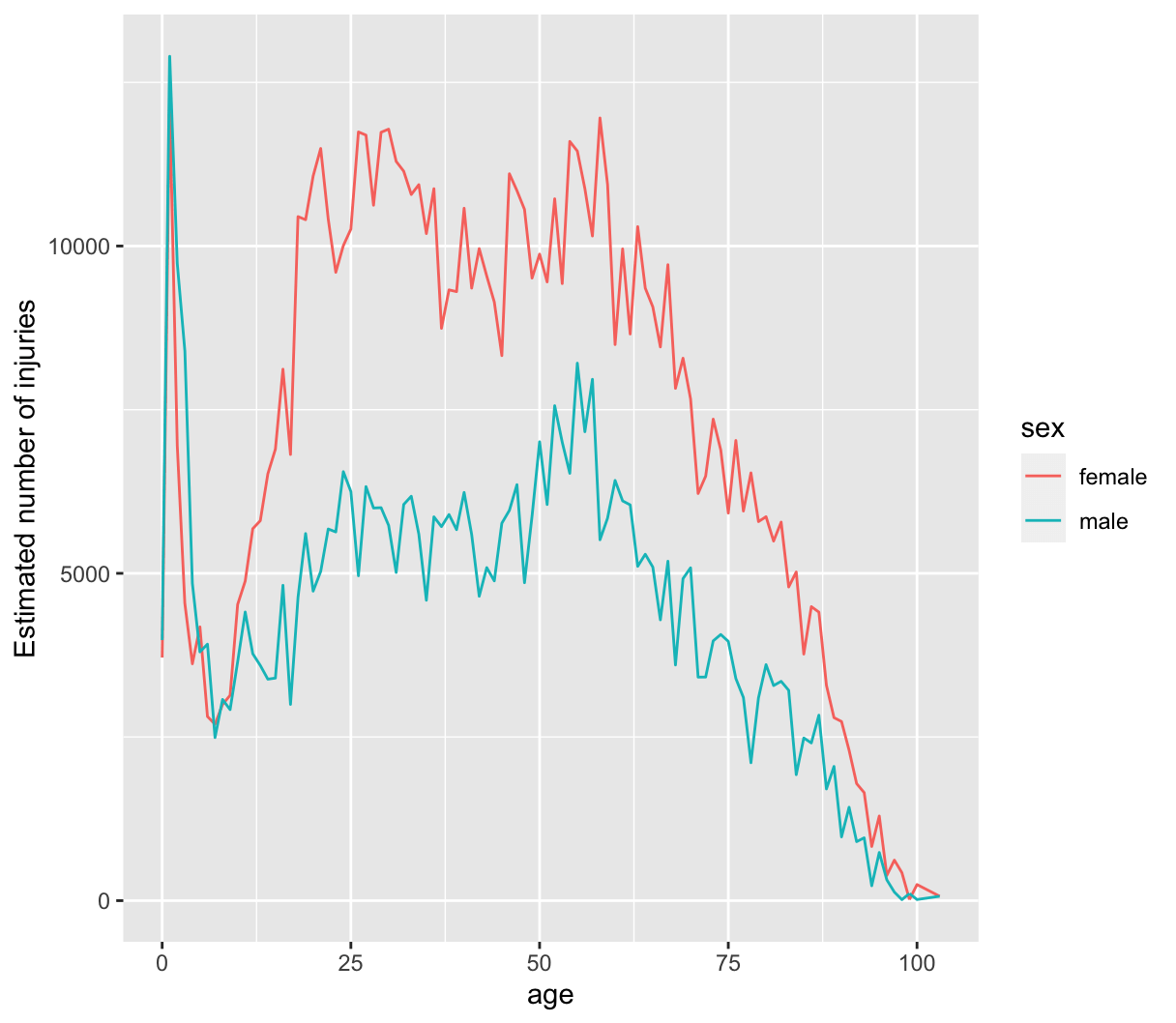
可以看到随着小孩学会走路,伤害的次数逐渐增多后逐渐平缓,有趣的是女性(高跟鞋的缘故?)受伤次数远远高于男性。由于老年人远远少于青年人,这种比较失衡,所以用受伤率来展示:
summary <- selected %>%
  count(age, sex, wt = weight) %>%
  left_join(population, by = c("age", "sex")) %>%
  mutate(rate = n / population * 1e4)
summary
# A tibble: 204 x 5
     age sex         n population  rate
   <dbl> <chr>   <dbl>      <dbl> <dbl>
 1     0 female  3714.    1924145  19.3
 2     0 male    3981.    2015150  19.8
 3     1 female 12155.    1943534  62.5
 4     1 male   12898.    2031718  63.5
 5     2 female  6949.    1965150  35.4
 6     2 male    9730.    2056625  47.3
 7     3 female  4542.    1956281  23.2
 8     3 male    8404.    2050474  41.0
 9     4 female  3618.    1953782  18.5
10     4 male    4845.    2042001  23.7
# … with 194 more rows
summary %>%
  ggplot(aes(age, rate, colour = sex)) +
  geom_line(na.rm = TRUE) +
  labs(y = "Injuries per 10,000 people")
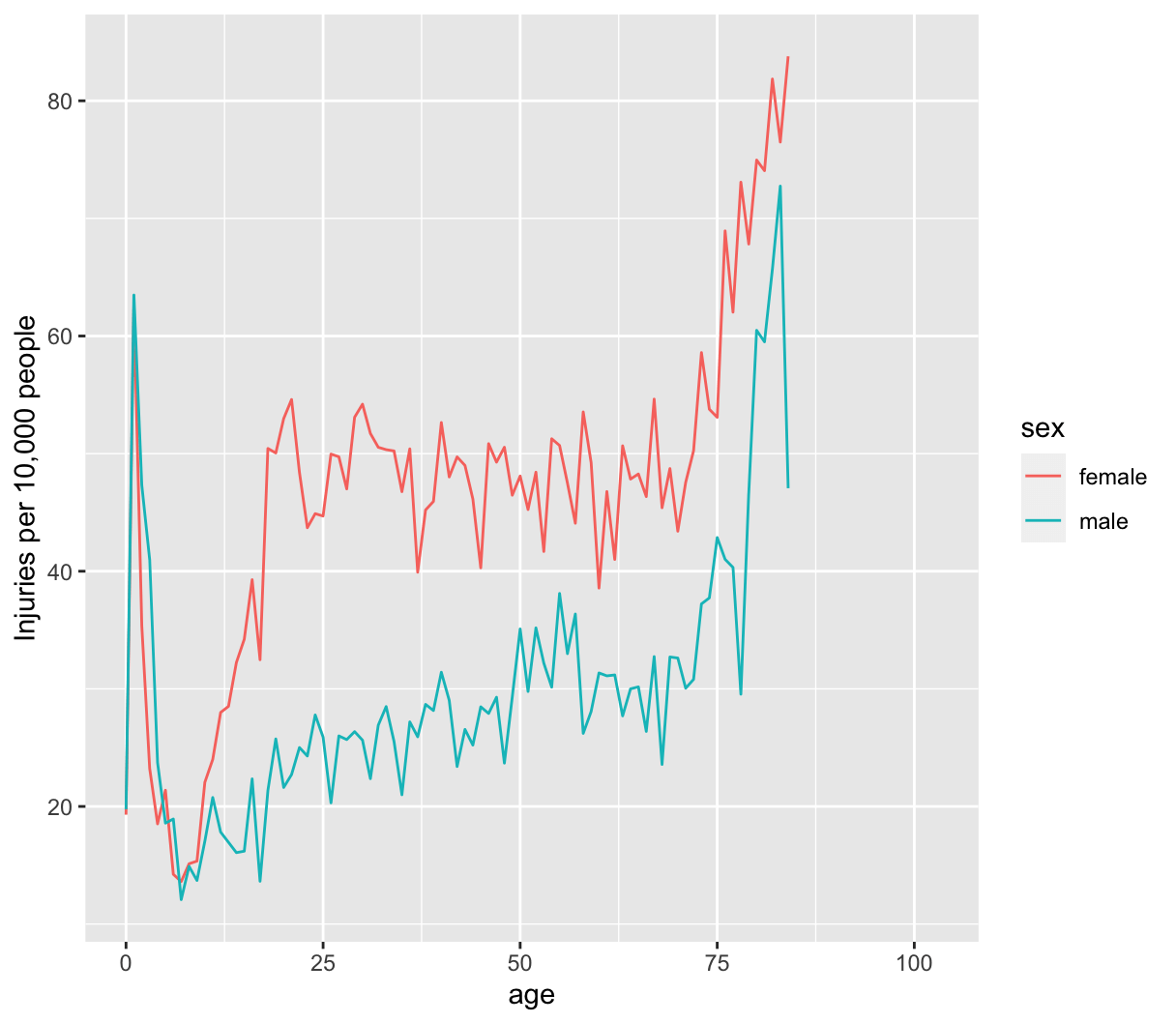
可以看出老年人受伤率十分高。
再看看具体的受伤诊断,随机抽取10行数据进行展示
-> selected %>%
   sample_n(10) %>%
   pull(narrative)
 [1] "56 YOM DX LT AC JOINT SEPARATION - S/P BIBEMS AFTER PT SLIPPED ONWATER,FELL DOWN 3 STEPS."
 [2] "LEFT WRIST FX. 61 YOF WAS WALKING DOWNSTAIRS WHEN SHE MISSED A STEP ANDFELL."
 [3] "39YOM KNEE PAIN- FELL DOWN STEPS"
 [4] "27YOF C/O RT ANKLE PAIN AFTER TRIPPING WHILE GOING DOWN STAIRS INVERTING ANKLE AT 2PM TODAY DX ANKLE SPRAIN"
 [5] "15YOF W/MOM PT FELL DN A STEP @HOME HITTING HER ANTERIOR KNEE , HAS HADPN SINCE X 1 HR PTA DX PATELLAR DISLOCATION, L"
 [6] "5 YOM FELL DOWN STEPS. DX FOOT CONTUSION"
 [7] "R HAND LAC/87YOWM TRIPPED DOWN A STAIR & SCRAPED R HAND ON THE WALL WHERE A NAIL WAS STICKING OUT. SUSTAINED LAC R HAND."
 [8] "61 YO F PT GOING DOWN STAIRS AT CHURCH FELT NAUSEA,DIZZY FELL HITTINGHEAD. DX CHI"
 [9] "15YOM WITH 2 SEIZURES AT HOME, ONE HE FELL DOWN STAIRS AND THE OTHERHE FELL OUT OF BED HITTING HIS HEAD ON FLOOR; HEAD INJURY, EPILEPSY"
[10] "*48YOF,UPPER BACKPAIN STARTED 2DAYS AGO FELL BACKWARDS ON STEPS W/PLAYING WITH DOG,HIT HEAD MAYBE,DX:MUSCULOSKELETAL PAIN"
App
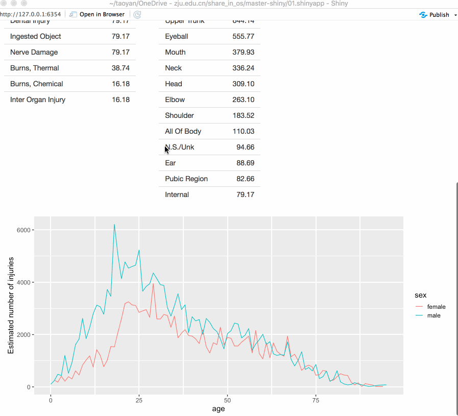
上面我们只探究了1842这一种,总共有30几种,我们不可能一一展示,这时创建一个Shiny App就可以方便我们探究任何一种伤害了。
根据上面分析的结果,先创建创建一个十分简单的app:只有一个输入,3个表格输出,1个图形输出
UI部分
ui <- fluidPage(
  fluidRow(
    column(6,
      selectInput("code", "Product", setNames(products$prod_code, products$title))
    )
  ),
  fluidRow(
    column(4, tableOutput("diag")),
    column(4, tableOutput("body_part")),
    column(4, tableOutput("location"))
  ),
  fluidRow(
    column(12, plotOutput("age_sex"))
  )
)
setName()将products$title赋值给products$prod_code,products$prod_code显示在UI,而products$title返回给server
server部分首先将selected以及summary写成reactive expression
server <- function(input, output, session) {
  selected <- reactive(injuries %>% filter(prod_code == input$code))

  output$diag <- renderTable(
    selected() %>% count(diag, wt = weight, sort = TRUE)
  )
  output$body_part <- renderTable(
    selected() %>% count(body_part, wt = weight, sort = TRUE)
  )
  output$location <- renderTable(
    selected() %>% count(location, wt = weight, sort = TRUE)
  )

  summary <- reactive({
    selected() %>%
      count(age, sex, wt = weight) %>%
      left_join(population, by = c("age", "sex")) %>%
      mutate(rate = n / population * 1e4)
  })

  output$age_sex <- renderPlot({
    summary() %>%
      ggplot(aes(age, n, colour = sex)) +
      geom_line() +
      labs(y = "Estimated number of injuries") +
      theme_grey(15)
  })
}
最后完整的app.R代码如下:
if (!require(shiny)){
  install.packages("shiny")
  library(shiny)
}
if (!require(vroom)){
  install.packages("vroom")
  library(vroom)
}
if (!require(tidyverse)){
  install.packages("tidyverse")
  library(tidyverse)
}
injuries <- vroom::vroom("../injuries.tsv.gz")
products <- vroom::vroom("../products.tsv")
population <- vroom::vroom("../population.tsv")

ui <- fluidPage(
  fluidRow(
    column(6,
           selectInput("code", "Product", setNames(products$prod_code, products$title))
    )
  ),
  fluidRow(
    column(4, tableOutput("diag")),
    column(4, tableOutput("body_part")),
    column(4, tableOutput("location"))
  ),
  fluidRow(
    column(12, plotOutput("age_sex"))
  )
)

server <- function(input, output, session) {
  selected <- reactive(injuries %>% filter(prod_code == input$code))

  output$diag <- renderTable(
    selected() %>% count(diag, wt = weight, sort = TRUE)
  )
  output$body_part <- renderTable(
    selected() %>% count(body_part, wt = weight, sort = TRUE)
  )
  output$location <- renderTable(
    selected() %>% count(location, wt = weight, sort = TRUE)
  )

  summary <- reactive({
    selected() %>%
      count(age, sex, wt = weight) %>%
      left_join(population, by = c("age", "sex")) %>%
      mutate(rate = n / population * 1e4)
  })

  output$age_sex <- renderPlot({
    summary() %>%
      ggplot(aes(age, n, colour = sex)) +
      geom_line() +
      labs(y = "Estimated number of injuries") +
      theme_grey(15)
  })
}

shinyApp(ui, server)
启动之后界面如下:
优化
主要是表格优化,因为显示太多不美观,这里定义一个函数用来显示出现频率最大的5组
count_top <- function(df, var, n = 5) {
  df %>%
    mutate({{ var }} := fct_lump(fct_infreq({{ var }}), n = n)) %>%
    group_by({{ var }}) %>%
    summarise(n = as.integer(sum(weight)))
}
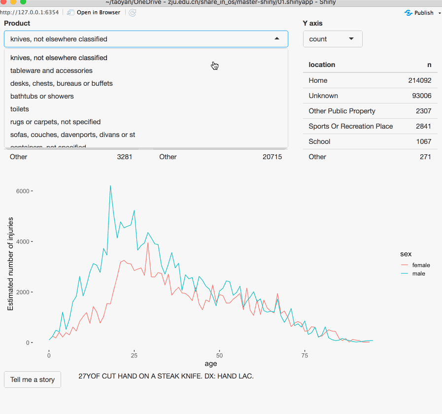
并将输出输出的宽度设置为最大,这样对齐美观。同时我们再添加一个选项,根据受伤率rate来绘制图形并显示具体的受伤过程narrative。
最终的app.R代码如下:
library(tidyverse)
library(vroom)
library(shiny)
if (!exists("injuries")) {
  injuries <- vroom::vroom("data/injuries.tsv.gz")
  products <- vroom::vroom("data/products.tsv")
  population <- vroom::vroom("data/population.tsv")
}

ui <- fluidPage(
  #<< first-row
  fluidRow(
    column(8,
           selectInput("code", "Product",
                       choices = setNames(products$prod_code, products$title),
                       width = "100%"
           )
    ),
    column(2, selectInput("y", "Y axis", c("rate", "count")))
  ),
  #>>
  fluidRow(
    column(4, tableOutput("diag")),
    column(4, tableOutput("body_part")),
    column(4, tableOutput("location"))
  ),
  fluidRow(
    column(12, plotOutput("age_sex"))
  ),
  #<< narrative-ui
  fluidRow(
    column(2, actionButton("story", "Tell me a story")),
    column(10, textOutput("narrative"))
  )
  #>>
)

count_top <- function(df, var, n = 5) {
  df %>%
    mutate({{ var }} := fct_lump(fct_infreq({{ var }}), n = n)) %>%
    group_by({{ var }}) %>%
    summarise(n = as.integer(sum(weight)))
}

server <- function(input, output, session) {
  selected <- reactive(injuries %>% filter(prod_code == input$code))

  #<< tables
  output$diag <- renderTable(count_top(selected(), diag), width = "100%")
  output$body_part <- renderTable(count_top(selected(), body_part), width = "100%")
  output$location <- renderTable(count_top(selected(), location), width = "100%")
  #>>

  summary <- reactive({
    selected() %>%
      count(age, sex, wt = weight) %>%
      left_join(population, by = c("age", "sex")) %>%
      mutate(rate = n / population * 1e4)
  })

  #<< plot
  output$age_sex <- renderPlot({
    if (input$y == "count") {
      summary() %>%
        ggplot(aes(age, n, colour = sex)) +
        geom_line() +
        labs(y = "Estimated number of injuries") +
        theme_grey(15)
    } else {
      summary() %>%
        ggplot(aes(age, rate, colour = sex)) +
        geom_line(na.rm = TRUE) +
        labs(y = "Injuries per 10,000 people") +
        theme_grey(15)
    }
  })
  #>>

  #<< narrative-server
  output$narrative <- renderText({
    input$story
    selected() %>% pull(narrative) %>% sample(1)
  })
  #>>
}

shinyApp(ui, server)
上面涉及到一些数据处理函数,我有段时间没用都生疏了,后面的再花点时间去学学数据处理函数,尤其是Tidyverse包里的。
我这里也提供一个 Shiny App用来查看浏览。
参考:https://mastering-shiny.org/basic-case-study.html