利用EMMAX进行GWAS分析
文件准备
利用EMMAX进行GWAS分析需要以下文件
基因型文件
基因型文件直接使用VCF进行过滤后得到,具体如下(我这里原始的VCF文件是test.vcf),过滤前先将染色体名称全部换为数值型(不然后续GWAS分析会报错的),同时添加SNP ID,这个比较简单就不讲了!
另外如果测序深度较低,可以基因型填补一下,按研究需要吧,这里就不进行了。
- 按基因型等位频率(0.05)以及缺失率(0.1)进行过滤
plink --vcf test.vcf --maf 0.05 --geno 0.1 --recode vcf-iid --out test.maf0.05.int0.9
生成test.maf0.05.int0.9.vcf文件
- 依据LD对标记进行筛选(这一步SNP必须有ID才行,GATK等软件生成的VCF文件是没有ID的)
plink --vcf test.maf0.05.int0.9.vcf --indep-pairwise 50 10 0.2 --out test.maf0.05.int0.9
产生test.maf0.05.int0.9.prune.in和test.maf0.05.int0.9.prune.out两个文件,in表示入选的标记,out表示被去除的标记,这两个文件都是只含有SNP ID,根据ID进行筛选
- 提取筛选结果
plink --vcf test.maf0.05.int0.9.vcf --make-bed --extract test.maf0.05.int0.9.prune.in --out test.maf0.05.int0.9.prune.in
- 将筛选后的数据转换为vcf格式
plink --bfile test.maf0.05.int0.9.prune.in --recode vcf-iid --out test.maf0.05.int0.9.prune.in
得到test.maf0.05.int0.9.prune.in.vcf基因型文件
- 将筛选后的文件转换为admixture数据格式用于群体结构分析
plink -bfile test.maf0.05.int0.9.prune.in --recode 12 --out test.maf0.05.int0.9.prune.in
得到test.maf0.05.int0.9.prune.in.ped用于admixture分析
- 将基因型文件转换为EMMAX格式
plink --vcf test.maf0.05.int0.9.vcf --recode 12 transpose --output-missing-genotype 0 --out test.maf0.05.int0.9 --autosome-num 90
得到tfam文件
- 群体亲缘关系分析
emmax-kin test.maf0.05.int0.9 -v -h -d 10 -o test.maf0.05.int0.9.BN.kinf

## 如果你下载的emmax软件是inter这个版本的,这里需要注意,命令有点不同
emmax-kin-inter64 test.maf0.05.int0.9 -v -d 10 -o test.maf0.05.int0.9.BN.kinf
群体结构文件
首先admixture群体结构分析,可以添加参数j,多线程
for i in {1..15}
do
admixture --cv test.maf0.05.int0.9.prune.in.ped ${i} -j48 >> log.txt
done
查看最佳分群
$ grep CV log.txt
CV error (K=1): 0.43802
CV error (K=2): 0.41492
CV error (K=3): 0.40182
CV error (K=4): 0.39723
CV error (K=5): 0.39281
CV error (K=6): 0.38899
CV error (K=7): 0.38640
CV error (K=8): 0.38434
CV error (K=9): 0.38301
CV error (K=10): 0.38156
CV error (K=11): 0.38050
CV error (K=12): 0.38006
CV error (K=13): 0.37869
CV error (K=14): 0.37795
CV error (K=15): 0.37830
K=14时CV值最小,所以最佳分群为14 K=14时候的Q矩阵用于后续分析。admixture产生的Q矩阵格式如下(前6行)
0.000010 0.864016 0.039019 0.000010 0.000010 0.000010 0.000010 0.000010 0.000010 0.096855 0.000010 0.000010 0.000010 0.000010
0.000010 0.135428 0.000010 0.039195 0.000010 0.192606 0.195391 0.062418 0.000010 0.124034 0.214463 0.000010 0.028383 0.008032
0.000010 0.613532 0.000010 0.043222 0.000010 0.000010 0.272258 0.000010 0.000010 0.000010 0.058748 0.000010 0.012151 0.000010
0.000010 0.419498 0.417594 0.000010 0.000010 0.000010 0.000010 0.000010 0.000010 0.000010 0.000010 0.090515 0.062396 0.009908
0.012456 0.045110 0.000010 0.000010 0.000010 0.021304 0.202956 0.049112 0.001099 0.455700 0.011129 0.093843 0.107251 0.000010
0.000010 0.071372 0.004548 0.000010 0.004779 0.000010 0.326421 0.009612 0.003101 0.211292 0.350671 0.000010 0.018153 0.000010
因为文件相对较小,手动添加表头信息,以及删除最后一列,保存14.Q用于后续分析,之后如下:
<Covariate>
<Trait> Q1      Q2      Q3      Q4      Q5      Q6      Q7      Q8      Q9      Q10     Q11     Q12     Q13
R4155   0.00001 0.864016        0.039019        0.00001 0.00001 0.00001 0.00001 0.00001 0.00001 0.096855        0.00001 0.00001 0.00001
R4156   0.00001 0.135428        0.00001 0.039195        0.00001 0.192606        0.195391        0.062418        0.00001 0.124034        0.214463        0.00001 0.028383
R4157   0.00001 0.613532        0.00001 0.043222        0.00001 0.00001 0.272258        0.00001 0.00001 0.00001 0.058748        0.00001 0.012151
R4158   0.00001 0.419498        0.417594        0.00001 0.00001 0.00001 0.00001 0.00001 0.00001 0.00001 0.00001 0.090515        0.062396
- 表型数据
EMMAX每次只能运行一个性状,格式与tfam格式类似,所以需要进行拆分转换,拆分前,需要将缺失值-999替换为NA。 最开始我的表型数据如下:
<Trait> day
R4155   184
R4156   181
R4157   181
R4158   182
R4159   170
R4160   179
利用R进行转换
tfam <- read.table("test.maf0.05.int0.9.tfam", header = F, stringsAsFactors = F)
tr <- read.table("test.trait.txt", header = T, check.names = F, stringsAsFactors = F)
tr <- tr[match(tfam$V1, tr$`<Trait>`),] ###把基因型文件样本顺序和表型文件样本顺序调整为一致
tr[tr == -999] <- NA
tre <- cbind(tr[,1], tr)
write.table(tre, file = "test_trait_emmax.txt", col.names = F, row.names = F, sep = "\t", quote = F)
转换后结果如下:
R4155   R4155   184
R4156   R4156   181
R4157   R4157   181
R4158   R4158   182
R4159   R4159   170
- 协变量文件
这里以群体结构作为协变量
tfam <- read.table("test.maf0.05.int0.9.tfam", header = F, stringsAsFactors = F)
admix <- read.table("14.Q", header = T, check.names = F, stringsAsFactors = F, skip = 1)
admix <- admix[match(tfam$V1, admix$`<Trait>`), ]
admix <- cbind(admix[,1], admix[,1], rep(1, nrow(admix)), admix[,-1])
write.table(admix, file = "test.emmax.cov.txt", col.names = F, row.names = F, sep = "\t", quote = F)
生成的协变量文件格式如下:
R4155   R4155   1       1e-05   0.864016        0.039019        1e-05   1e-05   1e-05   1e-05   1e-05   1e-05   0.096855        1e-05   1e-05   1e-05
R4156   R4156   1       1e-05   0.135428        1e-05   0.039195        1e-05   0.192606        0.195391        0.062418        1e-05   0.124034        0.214463        1e-05   0.028383
R4157   R4157   1       1e-05   0.613532        1e-05   0.043222        1e-05   1e-05   0.272258        1e-05   1e-05   1e-05   0.058748        1e-05   0.012151
R4158   R4158   1       1e-05   0.419498        0.417594        1e-05   1e-05   1e-05   1e-05   1e-05   1e-05   1e-05   1e-05   0.090515        0.062396
R4159   R4159   1       0.012456        0.04511 1e-05   1e-05   1e-05   0.021304        0.202956        0.049112        0.001099        0.4557  0.011129        0.093843 0.10725
GWAS运行
所有准备文件都有之后,就可以进行GWAS分析了
emmax -v -d 10 -t test.maf0.05.int0.9 -o test_emmax_cov -p test_trait_emmax.txt -k test.maf0.05.int0.9.BN.kinf -c test.cov.emmax.txt
最后生成的test_emmax_cov.ps就是我们需要的
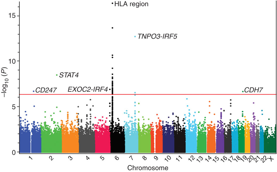
可视化
这里用qqman进行manhattan以及QQ图的绘制
#gwas_visualization.R
setwd("/database/pop-analysis-NY7/result/pop-structure/gwas")
if(!require(qqman)){
    install.packages("qqman")
    library(qqman)
}
if(!require(tidyverse)){
    install.packages("tidyverse")
    library(tidyverse)
}
gwas <- read.table("test_emmax_cov.ps", header = FALSE, stringsAsFactors = FALSE)
colnames(gwas) <- c("SNP","SE","P")
splite_chr <- function(data,c){
  c(str_split(data[c], pattern = "_")[[1]][1])
}
splite_pos <- function(data,c){
  c(str_split(data[c], pattern = "_")[[1]][2])
}
gwas$CHR <- apply(gwas,1,splite_chr,c="SNP")
gwas$BP <- apply(gwas,1,splite_pos,c="SNP")
gwas <- gwas%>%select(SNP,CHR,BP,P)
write.table(gwas,"gwas_emmax_test_for_vis.ps", col.names = TRUE, row.names = FALSE, quote = FALSE)
pdf("test_emmax_manhattan.pdf",width = 12,height = 6)
manhattan(gwas)
dev.off()
pdf("test_emmax_qq.pdf", width = 8, height = 6)
qq(gwas$P)
dev.off()
png("test_emmax_manhattan.png",width = 960,height = 600,type = "cairo")
manhattan(gwas)
dev.off()
png("test_emmax_qq.png", width = 800, height = 800,type = "cairo")
qq(gwas$P)
dev.off()
将上述脚本保存为gwas_visualization.R,之后在linux中运行
Rscript gwas_visualization.R
就可以得到我们需要的图
后续分析
后续还有很多分析,比如,显著位点的提取,关联基因的提取,关联基因的注释等等。。。。。。。